Vision Transformers

In this post we will cover high level concepts of using Transformers in Vision (ViT) tasks. We will follow the contours of ICLR 2021 paper by Google Brain - “An Image is Worth 16x16 Words Transformers for Image Recognition at Scale”. First we will cover the concept of ViT at a high level. Then we will do a quick recap of Transformers in general. And finally we will look at some implementation level details of Vision Transformers (ViT).

This post is divided into three parts:

1. Introduction
2. Background of Transformers
3. Vision Transformers (ViT)

1. Introduction

NLP (Natural Language Processing) has popularised the use of self-attention based Transformers as a way to go for scalable NLP tasks. Transformers have almost replaced RNN (Recurrent Neural Network) based architectures for NLP. Recently, Deep Learning research community has started to experiment with the use of Transformers in computer vision tasks as a replacement to the CNN (Convolutional Neural Network) based approaches. In NLP switching from RNN to Transformers offered a significant processing advantage in terms of parallel processing across the time (or sequence index) dimension. RNNs being recursive need the output of previous time step in the sequence to process the current sample/time-step. Transformers use a self attention approach to remove recursion and make it parallel.

However, CNNs are already inherently parallel and hence Transformers are not likely to offer any benefit similar to NLP’s switch from RNN to Transformers.

In the above paper on ViT, the authors show that ViT when trained on large amount of image data and then transferred to mid-sized or small image recognition data sets such as ImageNet, CIFAR-100 etc, ViT shows attains excellent results compared to state-of-art CNN based networks with substantially lesser computation resources to train.

2. Transformers

There are some excellent resources on Transformers and hence I will not attempt to go into all the details. I will just touch upon the basic high level concept behind Transformers with some pointers to learn more about it.

First let us define self-attention. Let us say our input is a sequence of words encoded as one-hot vectors. The one hot encoded vectors are converted into lower dimension word-embeddings. Word Embeddings convert a one-hot vector into a dense vector of lower dimension e.g. A word “deep” as represented by one-hot vector [0,0,…,1,0,…,0] is converted into a dense embedding vector of dimension say 128 [0.3, 0.2, -0.22, ….]. The embedding layer is learnt as part of the overall training task itself. In the embedding space, words with similar semantic meanings are closer than words with different meanings. The embedding space captures the semantic meaning of the words.

So after passing the one-hot vector sequence through the embedding layer, we have input as a sequence of embedding vectors representing the sentence. Let us say the example sentence is: “The cat is cute” where each word in the sentence is represented as a embedding vector of size k. Accordingly, the input sequence is \([x_1, x_2, ..., x_t]\). In self-attention, each embedding vector acts in three different ways to interact with the other vectors in the sequence. This interaction captures the influence or inter-dependence/covariance of the various words and allows words far apart in the sequence to influence each other just like the nearby vectors in the sequence. The three roles that each vector plays is called:

• Query
• Key
• Value

An input vector \(x_i\) is passed through three different k x k weight matrices:

\[\begin{align*} q_i = W_q x_i \; \; \; k_i = W_k x_i \; \; \; v_i = W_v x_i \end{align*}\]

All the key and query vectors are dot-product multiplied to get a t x t matrix \(W'\) where the element of this matrix is denoted by:

\[\begin{align*} w^{'}_{ij} = q_i^{T} k_j \end{align*}\]

The weight matrix is softmaxed over each row individually, i.e., across the columns for each row.

\[\begin{align*} w_{ij} = softmax(w^{'}_{ij}) \; \; \text{over dimension 1.} \end{align*}\]

The i-th row of softmaxed weight matrix \(W\) signifies the weights to be used for computing the output \(y_i\) of self-attention block. The row contains the relative influence (weight) that each of the words in the sequence have for the i-th output.

Next the vectors \(v_i\) are combined together with i-th row of the matrix \(W\) to produce the i-th output \(y_i\).

\[\begin{align*} y_i = \sum_{j} w_{ij} v_j \end{align*}\]

This is the basic essence of self-attention, where the output is a weighted sum of all inputs using the key-query-value construct as explained above.

Figure 1: Self attention schematic. source

There are a few additional details such as scaling the dot-products and using multiple self-attention heads which you can read about in the original paper “Attention is all you need”. There is a great blog that you can follow which relooks at the Transformer architecture and I think it is one of the best explanation on Transformer. You can find the blog here.

A Transformer is more than just self-attention. We use self-attention to first construct a Transformer Block as shown in figure 2. *Residual connection” is added around the self-attention block. This is then passed through a layer-norm block followed by multiple MLP layers which also have residual connections. And the output is finally passed through another layer-norm block.

Figure 2: Single Transformer block. source

Multiple such Transformers are connected in series. A very nice and easy to follow Transformer architecture (mini version of GPT) implementation in PyTorch by Andrej Karpathy can be found here.

3. Vision Transformers

Vision transformer approach is very similar to the one followed by NLP Transformer models. We first divide the images into patches say 14x14 patches or something like that. Each patch is passed through a CNN with filter size equal to the patch size and number of output channels equal to “k” the embedding vector size. The embedded sequence is further augmented with position embeddings to encode the position of each image patch. Just like one-hot vectors for words, the position embeddings are also created from one-hot position vectors.

The sequence is then passed through a standard Transformer Block as shown in the right of figure 3. You may notice that the Transformer block is fairly similar to the one we saw on figure 2 except for the position of the layer-norm block position.

The output of the Transformer block is then passed through a standard MLP (Multilayer perceptron network) to output the probability of the image belonging to a image class. This is the standard image classification construct.

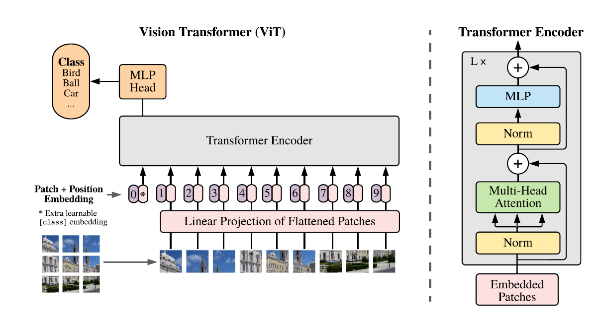
Figure 3: Vision Transformer (ViT) architecture

A nice PyTorch implementation of ViT can be found in here. The repository contains PyTorch implementations of various image models.

4. Conclusion

These are still early days of Vision Transformers and many new papers have been published after the first one by Google Brain. While, the current industrial use of Image and computer vision is dominated by CNN based architectures, Vision Transformers have shown an initial promise. Will Transformers replace CNN for vision tasks is still not clear. It is early days but exciting times to see where will Transformers lead the computer vision field to.

I hope you liked the post. You can reach me at linkedin.